Real Time Rendering Experiments
These experiments were made with THREE.js for the rendering course at the University Paul Sabatier in 2017.
Loop Subdivision
This project implements the loop subdivision for triangular based meshes. Three new points are created on the edges of each triangle after each iteration and old vertices are moved according to their surroundings.
The code is subdivided into four main steps:
- Data pre-processing
- Creation of data structures for edges which include adjacent faces
- Add adjacent vertices to each vertex
- New points calculation on edges
- 12/16 of the new point position come from vertices of the edge
- 4/16 come from the opposite vertices of the two adjacent faces
- Recalculate the new position of already existing vertices
- A weight is assigned to the already existing vertex and to each adjacent vertices with a formula which sum to 1
- New geometry is created
- Four new faces are created per triangle thanks to new vertices previously calculated
For example the cube, Figure 1, with the starting meshes.
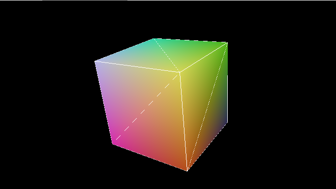
Which gives us after a step of the subdivision, Figure 2, in red the studied triangle, in blue the newly created edges from the new points and in cyan the old triangle.
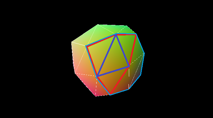
The number of step of subdivision can be selected in between 0 to 9. The user can also select another starting geometry and if the wireframe is shown.
For the moment, the coded algorithm does not include edges special cases so all geometries are closed ones.
Implicit Surfaces
The marching cube algorithm allows the visualization of implicit surfaces. Actually, they are characterized from a mathematical equation so they cannot be rendered directly to the screen.
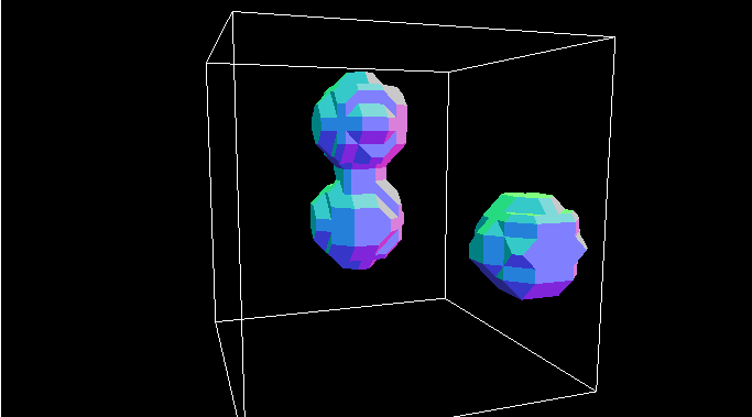
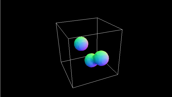
The space is divided into smaller cubes. Here the initial space is a cube of size 1x1x1 which is divided into 12x12x12 smaller cubes. The sum of the mathematical functions of each implicit surface is calculated for each vertex of the newly divided space. Here three metaballs are present. This will allow us to deduce which vertices are inside or outside of our threshold.
For each configuration of the vertices of the cube in the inside or outside of our implicit surface, there are 15 possible cases (and their symmetric), see Figure 3. The 256 possible cases are stored in a table. This table gives the triangles to draw from the half-edge for each a cube.
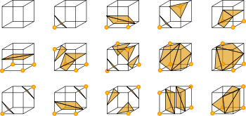
Source: Wikipedia
We calculate a value coded on eight bits from the vertex, this gives us the index to use in this table to gather triangles to draw in the current small cube.
At this point, the results are simple low poly spheres as shown on Figure 4.
Value in-between vertices are linearly interpolated to approximate the position where the function exceeds our threshold on each edge.
Value in-between vertices are linearly interpolated to approximate the position where the function exceeds our threshold on each edge.
Fast Approximated Anti-Aliasing
The FXAA is an algorithm created by NVIDIA.
The algorithm is implemented thanks to a shader which uses the texture of a first rendering of the scene. It’s really fast as it based on a study of the luminosity of the objects and brief edge detection, whereas the other anti-aliasing algorithms are based on multiple renderings.
On figure 6 and 7 are shown the different renderings accessible from the example page and the explication in regards to the algorithm.
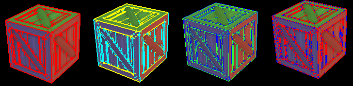
FXAA_DEBUG_PASSTHROUGH: selected pixels to be treated are shown in red, these are the ones supposed to be on an edge where the luminosity gradient is important but also where the luminosity is important enough for the human eye. FXAA_DEBUG_HORZVERT: pixels are sorted between the ones on a horizontal edge in yellow and vertical edge in cyan. FXAA_DEBUG_PAIR: “pair” of pixels is denoted in different colour depending on the direction of the half pixel displacement (90° to the edge). FXAA_DEBUG_NEGPOS: shows the direction in which the algorithm extended the most before encountering a bigger gradient of luminosity, thus the end of the current edge (red for negative and blue for positive).
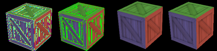
FXAA_DEBUG_OFFSET: mix between FXAA_DEBUG_PAIR and FXAA_DEBUG_NEGPOS. FXAA_DEBUG_LOWPASS: show where the algorithm used a local blur filter to calculate the value of the new value of the pixel in green and the value calculated with the algorithm in red.
Screen-Space Ambient Occlusion
SSAO algorithm uses the depth buffer. After a first render pass we get the rendered scene and its associated depth map.
The algorithm follows three main steps:
- Normal map estimation
- Using the depth map it is possible to estimate the surface normal for each pixel of the image
- Taking the normal and depth into account, an hemisphere of 16 points is generated around the studied point
- For each of the generated point, its depth is compared with the one in the depth map
- If it is inferior, then the point is considered obscured
- The difference with the depth map value is also calculated, if it goes over a certain threshold it isn't taken into account to avoid distant objects to occult each other
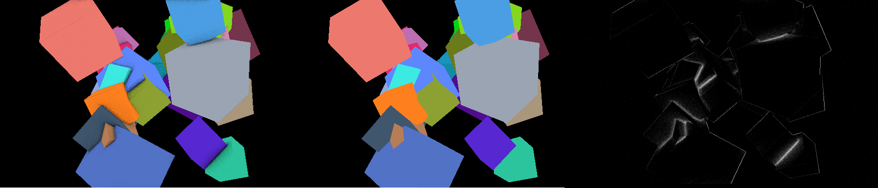
The algorithm can be completed by applying a Gaussian blur to the occlusion map in order to reduce the noise coming from the random sampling.